on
Tags: finance, Stan, Bayes
Bayesian Style Analysis
Sharpe’s style analysis remains a workhorse took for people in industry who are looking to figure out what a fund’s risk exposures are while constraining these exposures to long-only positions. This is typically implemented as a quadratic programming problem that finds the optimum (least squares) solution under constraints.
But we could also think of it as a regression with parameter regularization via informative priors. Indeed, Sharpe himself discusses this as a means to improve out of sample fit:
It is important to recognize that [$R^2$] indicates only the extent to which a specific model fits the data at hand. A better test of the usefulness of any implementation is its ability to explain performance out-of-sample. For this reason it is important to consider not only the ability of a model to explain a given set of data but also its parsimony. Other things equal (e.g. R-squared values), the fewer the asset classes, the more likely is the model to represent continuing fundamental relationships with predictive content.
And subsequently,
The addition of constraints reflecting the fund’s actual investment policy causes a slight reduction in the fit of the resulting equation to the data at hand (i.e., a decrease in R-squared to 92.22%). Now, however, the coefficients conform far more closely to the reality of the fund’s investment style, making the resulting characterization more likely to provide meaningful results with out-of-sample data.
In other words, we want a model that we know to be consistent with the investment policy of a manager (we have external knowledge we bring to bear on the problem) and we want to replicate their forward-looking performance as best we can while still adhering to their policy.
A Bayesian Interpretation
We can formulate this optimization problem in terms of a generative Bayesian model. Given a matrix of $k$ factor returns $X$ measured $t$ times and a vector of fund returns $R$ (in log-space) we can formulate the problem as
$R = \beta X + \epsilon$
where there is a point-mass prior on the sum of $\beta$, e.g.
$P(\Sigma_{i=1}^k \beta = 1) = 1$
and a uniform constraint on each $\beta_i$ such that
$\beta_i \sim Uniform(0,1)$
for each $i \in {1, …, k}$.
Now that we have a Bayesian formulation of the model, it is completely straightforward to do things like estimate confidence intervals of the style weights, which are going to be inherently asymmetric. This is a serious gap in the traditional treatment of the optimization problem, but in the Bayesian framework we can just explore the posterior with MCMC, just like any other model.
In other words, if we want to quantify our uncertainty about each parameter in the style analysis (as in the linked article) we don’t need an approximate formula for symmetric standard errors. We can also easily accomodate the tails of the parameter distribution where they rub up against the informative prior. It is interpreted the exact same way any other posterior disribution is, and we can simply quantile the MCMC draws to get the estimate.
Similarly, if we didn’t believe a strategy to be fully invested in the asset classes we were measuring it against, we could weaken our prior formulations to accomodate that information. In other word, we can just treat this like any other model, and better diagnose when and if our model is going wrong.
Coding the model
I’m using Stan to code the model. The simplex statement implies a sum-to-1 constraint (and I believe it forces positive weights), and the uniform(0,1) prior implies constraints on each individual $\beta$. While I’m pretty sure the simplex statement implies positive weights I’m not certain, so I’m just going to add in the call to uniform(0, 1) to be safe. Before fitting the model, I transform the raw returns into log returns because this linearizes the return series (which otherwise compound geometrically and are constrained at -1).
data {
  int<lower=0> N; // length of time
  int<lower=0> K; // number of factors
  matrix[N, K] X; // factor matrix
  vector[N] R; // vector of returns
}
parameters {
  real alpha;
  simplex[K] beta; // beta parameters, simplex implies sum-to-1
  real<lower=0> sigma; // variance parameter
}
model {

  // positive and maximum constraints
  for(k in 1:K) {
    beta[k] ~ uniform(0, 1);
  }

  // linear regression model
  R ~ normal(alpha + X * beta, sigma);
}
generated quantities {
  vector[N] R_rep;
  for(n in 1:N) {
    R_rep[n] = normal_rng(alpha + X[n,] * beta, sigma);
  }
}
Something we get for free with this approach is other quantities of interest we would want froma a statistical model: get standard errors, correlations, etc. We don’t need to derive formulas for approximate forward looking variances of asset betas (and thus asset weights). We can just use the posterior distribution.
Secondly, once we frame the problem this way, we can easily add more prior information or weaken prior information as might be appropriate. For example, if we know a fund has leverage, we might put a prior on the sum of the weights that takes into account the maximum amount of leverage they are allowed by policy, weakening the specific sum of the weights.
Finally, we can see some of the pathologies induced by the prior when we examine the poserior draws. These aren’t inherently something terrible, but we see that the mean and median of the posterior are quite far from the mode! If we were forced to choose a portfolio to replicate the strategy given the style weights, how would we choose?
So to start, let’s compare our fit to the implementation from the FactorAnalytics R package that contains a pre-built function that solves the problem using quadratic programming. I’m going to grab some relevant fund and index data using the quantmod package, that uses the Yahoo and/or Google Finance APIs to get daily price series. Because I know the fund fairly well, let’s test this with AMCAP Fund class A.
Here are the functions I’m using to grab relevant index data. I’ve decided to use daily closing prices for my return series, and I calculate the returns using the PerformanceAnalytics package.
library(quantmod) # yahoo finance
library(PerformanceAnalytics) # performance calculations
library(magrittr) # ceci n'est pas une pipe
library(rstan) # for fitting the stan model

get_price <- function(symbol) {

  sym_name <- gsub("[^A-Za-z]", "", symbol)
  sym <-
    getSymbols(symbol, auto.assign = F)

  colnames(sym) <- gsub(paste0(sym_name, "."),
                         "",colnames(sym), fixed = T)

  sym <- sym[,"Close"]
  colnames(sym) <- sym_name
  sym[]
}

get_prices <- function(symbols) {
  Reduce(merge, lapply(symbols, get_price))
}

# S&P 500, Russell 2k, 90 day treasuries,
# 5 year treasuries, 10 year treasuries, 30 year treasuries,
idx <- c("^GSPC", "^RUT", "^IRX",
         "^FVX", "^TNX", "^TYX")

# a couple random mutual funds
# AMCAP Fund A and Wasatch-Hoisington US Treasury Fund
fund <- c("AMCPX", "WHOSX")

calc_returns <- function(symbols) {
  get_prices(symbols) %>%
    .[complete.cases(.),] %>%
    Return.calculate(.)
}

idx_returns <- calc_returns(idx)

fund_returns <- calc_returns(fund)
This gives us a matrix of index returns and fund returns, which we then want to pass to Stan for sampling (and to FactorAnalytics for optimizing). I built a function that converts this to data for the Stan script above before being passed through for optimization or MCMC sampling.
# function for turning this into
# a list that our stan model can use
make_standata <- function(fundRet, idxRet) {
  # save which is which
  idxNames <- colnames(idxRet)
  fundNames <- colnames(fundRet)

  # only use periods where they both have returns
  joint_ret <- merge(idxRet, fundRet) %>%
    .[complete.cases(.),]

  list(
    N = nrow(joint_ret),
    K = length(idxNames),
    X = as.matrix(log1p(joint_ret[,idxNames])),
    R = as.vector(log1p(joint_ret[,fundNames]))
  )
}

# compile model
# requires the stan file to be
# in the working directory
style_reg <- stan_model("bayesian-style.stan")

# create data
# daily returns
amcap_style_data <-
  make_standata(fund_returns$AMCPX,
                idx_returns)

# weights should be the same
FactorAnalytics::style.fit(log1p(amcap_style_data$R),
                           log1p(amcap_style_data$X))

# MCMC sampling
amcap_fit <- sampling(style_reg, data = amcap_style_data)
Here is the output from the FactorAnalytics optimization:
| GSPC | RUT | IRX | FVX | TNX | TYX |
|---|---|---|---|---|---|
| 0.89 | 0.07 | 0 | 0 | 0 | 0.04 |
And here is the output from stan::optimizing() (once I set up the tuning parameters to be a little more sensitive to the relative gradient and value changes of the objective function).
| GSPC | RUT | IRX | FVX | TNX | TYX |
|---|---|---|---|---|---|
| 0.89 | 0.07 | 0 | 0 | 0 | 0.04 |
So we have agreement! But what I particularly like about this approach is that we can get direct confidence intervals for our parameters via MCMC sampling. I would speculate that fitting this model with 10 years of daily returns over 10 years using Metropolis-Hastings this might have taken a while, especially if there was weird geometry induced by the priors, but with Stan and HMC it’s pretty fast. The whole thing (with simulated posterior draws) takes about 2 minutes. We also end up with the same answer (in expectation),
Inference for Stan model: bayesian-style.
4 chains, each with iter=2000; warmup=1000; thin=1;
post-warmup draws per chain=1000, total post-warmup draws=4000.

                mean se_mean   sd     2.5%      25%      50%      75%    97.5% n_eff Rhat
alpha           0.00    0.00 0.00     0.00     0.00     0.00     0.00     0.00  4268    1
beta[1]         0.89    0.00 0.01     0.87     0.88     0.89     0.90     0.91  1977    1
beta[2]         0.07    0.00 0.01     0.05     0.06     0.07     0.08     0.09  1690    1
beta[3]         0.00    0.00 0.00     0.00     0.00     0.00     0.00     0.00  3507    1
beta[4]         0.00    0.00 0.00     0.00     0.00     0.00     0.00     0.00  3485    1
beta[5]         0.00    0.00 0.00     0.00     0.00     0.00     0.00     0.00  3937    1
beta[6]         0.04    0.00 0.00     0.03     0.03     0.04     0.04     0.05  4493    1
The indexes are listed in the same order as the previous column names. We can also visualize this by plotting kernel density estimates of the parameters.
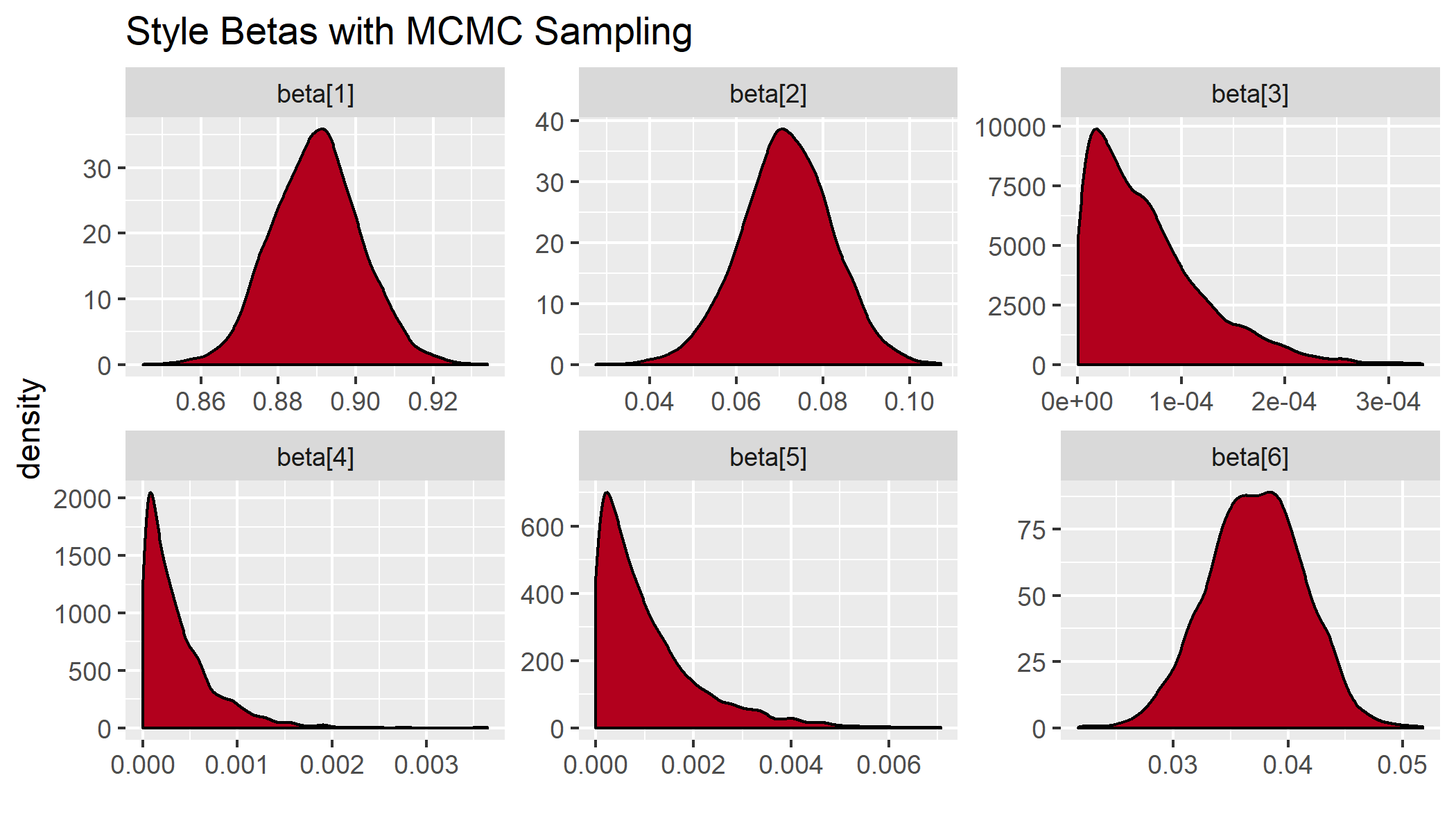
In this case it looks like the confidence intervals of the important variables are fairly symmetric, but we already see some asymmetries for the variables that butt up against the prior.
This problem gets worse if I include highly correlated indexes that contain large blocks of the same underlying securities. For example, if I include correlated assets that make up the majority of the portfolio, like the Russell 1000 Value, the Russell 1000 Growth, and the S&P 500, I get some weird-looking results where the posterior mode is no longer equivalent to the expectation.
Here’s the solution via FactorAnalytics::style.fit():
| GSPC | RLV | RLG | RUT | IRX | FVX | TNX | TYX |
|---|---|---|---|---|---|---|---|
| 0.02 | 0.23 | 0.67 | 0.04 | 0 | 0 | 0 | 0.04 |
When I run the code via rstan::optimizing(), which uses L-BFGS to compute the maximum posterior draw, I get something very similar to the quadratic programming approach. That said, the posterior mode is on a knife’s edge, with different initial values getting substantially different weights (sometimes as extreme as a weight of 1 on S&P, and 0 on everything else).
| GSPC | RLV | RLG | RUT | IRX | FVX | TNX | TYX |
|---|---|---|---|---|---|---|---|
| 0.01 | 0.24 | 0.67 | 0.04 | 0 | 0 | 0 | 0.04 |
But here is the full posterior fit with MCMC sampling:
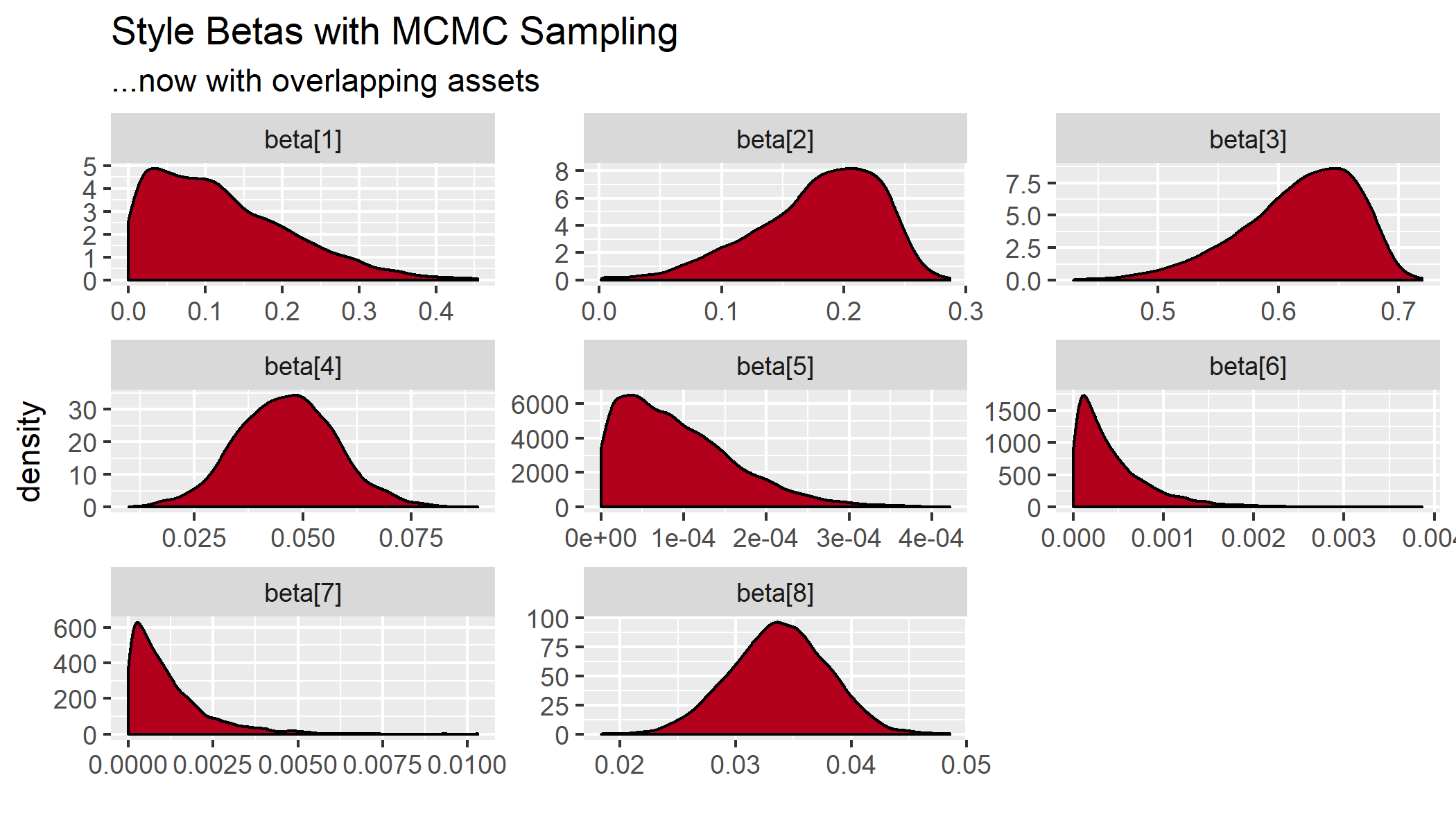
Where the betas are in the same order as the table previous. That gives us the S&P 500, the Russell 1000 Value, the Russell 1000 Growth, the Russell 2k, and several treasury indexes.
We can also look at the quantiles of the posterior weights, which tell the same story.
Inference for Stan model: bayesian-style.
4 chains, each with iter=2000; warmup=1000; thin=1;
post-warmup draws per chain=1000, total post-warmup draws=4000.

     mean se_mean   sd 2.5%  25%  50%  75% 97.5% n_eff Rhat
GSPC 0.12       0 0.09 0.01 0.05 0.11 0.18  0.33  1367    1
RLV  0.18       0 0.05 0.07 0.15 0.19 0.22  0.25  1326    1
RLG  0.62       0 0.05 0.51 0.59 0.62 0.65  0.69  1415    1
RUT  0.05       0 0.01 0.02 0.04 0.05 0.05  0.07  1460    1
IRX  0.00       0 0.00 0.00 0.00 0.00 0.00  0.00  2767    1
FVX  0.00       0 0.00 0.00 0.00 0.00 0.00  0.00  3757    1
TNX  0.00       0 0.00 0.00 0.00 0.00 0.00  0.00  3344    1
TYX  0.03       0 0.00 0.03 0.03 0.03 0.04  0.04  4994    1
So the quadratic programming approach gives us something close to the posterior mode, but not at all close to the the expectation. The posterior for the S&P 500, for example, has a mode close to 0.01, and a mean close to 0.11. I suppose this is nothing more than a warning sign for someone not to assign too much weight to the constrained optimization in the case of highly correlated indexes that push each other around.
At the very least, it seems to like we should either shy away from using correlated assets when using the optimization approach or introduce stronger prior information about the coefficients of the specific asset weights in order to help work through this issue. Regardless, the MCMC method will return the mode, the median, and expectation, which helps to elucidate just how extreme this problem can be. Since traditional style analysis so often involves correlated assets, this approach can properly determine how uncertain we should be about the various weights.
From a decision-theoretic perspective, it also makes sense to look at exactly how uncertain the parameter values. It could also be that going with many sets of indexes has such similar tracking error it ceases to really matter how to move forward. What I particularly like about treating this as a Bayesian model is that all these questions are easily and consistently pursued.
Another thing that the fully specified posterior + likelihood lets us do is draw from the full posterior predictive distribution. You can see in the generated quantitites section of the Stan code that for each draw from each parameter I am generating a draw for my expected return, with errors drawn from the distribution I chose for the likelihood. We can see how well the model is calibrated with visual checks that compare the distributions. If we take 40 draws from the posterior for the same time series as we trained it on, we see that the error term used by the likelihood we chose (or perhaps the assets we picked) doesn’t properly pick up the frequency at the central tendency because it overfits the tails of the distribution.

We might be able to fix this by taking into account volatility clustering in the residuals through either a GARCH process or stochastic volatility model. Alternatively, we may just not be capturing the underlying asset correctly. Regardless, the assumption of normally distributed errors is ok, but not perfect, with our constrained regression.
Summing Up
This framework is far more general than just Sharpe’s style analysis. Indeed, it seems like almost any constrained structural problem could be formulated with these types of priors. Maybe in some future work I’ll get to discuss this in a broader context, but hopefully this is enough inspiration to use MCMC sampling to check whether your constraints are introducing unexpected (or unaccounted for) correlations in your parameters that could bias your maximum likelihood (or maximum approximate posterior) point estimates.
In an upcoming post I’ll talk about playing around with the model in order to accomodate non-traditional strategies (e.g. constrained leverage or long-short), help select between correlated predictors and induce sparsity, and take into account volatility clustering in the time series of the various assets under consideration. I’ll also talk through formulating the problem with soft constraints and see whether that makes a substantial difference in the stability of the convergence of the models.