on
Tags: finance, meta-analysis, Bayes
Analysts & Meta-Analysts
One thing I’ve been thinking about is how to aggregate financial analyst forecasts. The essential job of an analyst is to forecast the price of a security (perhaps over different windows). Then they distill that to a recommendation (buy, sell, etc.). We might expect these analysts to be more or less sensitive to different sources of information, and also to have different default positions for their expectations of how a company will do. There is one true future price that is going to arise as a function of changes in expectations of future earnings, price momentum, sales, or whatever. Some mix of characteristics.
Even more vague is how to properly aggregate forecasts for asset classes as a whole! Different companies come out with “capital market assumption” forecasts that are based on entirely opaque models or in the worst case scenario just a gut feeling. The Bayesian in me wants people to give some kind of distribution on both their expectation of the mean and the variance, but ultimately these types of “expert” (e.g. non-model-based) forecasts are hard enough as is. That makes it difficult to appropriately propogate the uncertainty in the forecasts into the aggregated forecasts.
A motivating example
As a simple example (this is something people actually do), we might just take an average of the forecasts for the mean and the variance. Then those get plugged into our mean-variance optimizer, and we end up with some asset allocation. But suppose that we have 3 analysts that were asked to give point forecasts about the returns and standard deviations of some asset class over the next year.
| Metric | Amy | Bob | Carla |
|---|---|---|---|
| Mean | 0.08 | 0.06 | -0.05 |
| Std. Dev. | 0.01 | 0.02 | 0.06 |
Carla clearly expects some kind of correction, Bob expects close to average returns, and Amy thinks there’s going to be very good risk adjusted returns. Does the volatility of Carla imply greater uncertainty? Or just bad risk-adjusted return? Perhaps Carla is actually very confident about the average, but also thinks that volatility is going to spike!
Now even without a direct measure of uncertainty in their predictions of the mean, we still need to take into account the level of disagreement between the analysts in our forecast of the asset classes returns. We might assume that returns $y$ are given by
$y = \mu + \epsilon$
and the mean is given by some aggregated mean around the forecast. Suppose that we use the average of the three predicted standard deviations (0.03) as our volatility forecast, e.g. $\epsilon \sim Normal(0, 0.03^2)$, and the standard error of a naive mean estimator as our uncertainty about $\mu$. In other words
$\mu \sim Normal(0.03, \dfrac{0.07^2}{3})$
Then $y_{forecast} \sim Normal(0.03, \dfrac{0.07^2}{3} + 0.03^2)$, or a standard deviation of about 0.05 for the forecasted $y$. This would be a very simple thing to do, but is also likely to underestimate the uncertainty in the forecasts. We’ll see why in a second.
Analysts and Meta-analysis
Meta-analysis
Meta-analysis, or the process by which we aggregate conclusions of different studies, has a very similar problem as CMA forecasts. In an ideal setting we would have access to the underlying data and modeling process, and we could aggregate at that level, adjusting for differences in study design along the way. However, we often only have access to the rough measurements that the studies have published.
So we might only have access to a series of published means and standard errors for an estimate of some kind of treatment effect. At the same time, the actual structure of the studies and differences in the underlying studied populations might be entirely obscured. One of the canonical models for how to aggregate these effects assumes that each measured effect is randomly drawn from some distribution.
In other words while the measured treatment effect in study $i$ is given by
$\hat{\tau_i} \sim Normal(\tau_i, \sigma_i^2)$
where $\sigma_i$ is the standard error of the measured effect in study $i$, we also presume that the unobserved true $\tau_i$ is given by
$\tau_i \sim Normal(\tau, \sigma^2),$
where $\sigma^2$ is the variance of the meta-distribution that the heterogenous treatment effects are drawn from and $\tau$ is the unobserved true effect being measured by the studies. So what we really want to know if we were to implement some intervention that would impact some variable of interest is $\tau$, representing the latent treatment effect that generated our heterogenous measurements.
Now this normal distribution seems like a fiction, and in some ways it is, but it also is a useful assumption that allows us to actually aggregate our estimates, all the while propogating our uncertainty of each studies measurements forward into our aggregate effect estimate. Another way to think about this is that without additional information about each study, the differences between them are ignorable. Thus we can exchange one study for another without messing up our analysis. If we had more information about the various studies we would certainly want to model them!
Analysts
Analysts or other forecasters have largely the same issue. J.P. Morgan (or Goldman Sachs, or an internal team for a buy-side firm) comes out with a forecast for equity returns for the next year, but we don’t really know what type of information they are using to forecast it. We don’t have the underlying data that would allow us to weigh this forecast vs. another, or my own. It is also fair to say that almost every CMA forecast is pretty terrible.
If I were to run a firm that employed several analysts, I would not only ask what the average of their forecast was, but also how certain they were about their point prediction. For example, I might ask “What range will this coming year’s return fall into 90% of the time?” and then use that to calibrate a standard error for a normal (or log-normal) distribution. If we don’t have that, we could just calibrate the errors with their residuals from previous forecasts.
Obviously analysts forecast all sorts of things–sometimes you might get a model of earnings or a buy/sell/hold rating–but to keep these simple let’s keep working with returns. As an example, we might look at the types of capital market assumption reports that come out from investment banks on an annual basis.
Now let’s imagine that I’ve already done this, and we have a set of some analysts and the associated standard errors of their predictions. It’s important to remember that, as above, these are not the same as the predicted volatility of the asset, but instead uncertainty about the mean.
| Analyst | Point Prediction | Standard Error |
|---|---|---|
| 1 | 0.08 | 0.05 |
| 2 | 0.05 | 0.02 |
| 3 | 0.02 | 0.10 |
| 4 | -0.05 | 0.03 |
| 5 | 0.02 | 0.02 |
| 6 | 0.03 | 0.10 |
| 7 | -0.01 | 0.12 |
| 8 | 0.09 | 0.02 |
Fitting the model
Let’s do this in R. The baggr package is designed for Bayesian meta-analysis modeling, which allows us to fit the meta-analysis model described above.
library(baggr) # bayesian meta-analysis models
library(quantmod) # get returns for things
library(data.table) # GOAT data package
library(ggplot2) # plotting

# let's number these nameless analysts, and give them
# each a standard error and average prediction
us_eq_forecasts <- data.table(
analyst = 1:8,
avg_pred = c(0.08, 0.05, 0.02, -0.05,
                0.02, 0.03, -0.01, 0.09),
se_pred = c(0.05, 0.02, 0.1, 0.03,
            0.02, 0.1, 0.12, 0.02)
)
By default, the baggr package assumes extremely weak priors. This can be ok if you have a lot of data (in this case analyst forecasts), but in such a small data setting I would recommend something a little bit more informative.
In this case I’m imposing a prior on the latent mean that takes into account the fact that US Equity Markets are historically up 7% a year. I’m also incorporating a large amount of uncertainty around that mean (e.g. 20%), which is weaker than necessary. In this sense we might call this type of prior “weakly informative” because while it contains information about the location and scale, it is not so strong as to truly inform the data.
The standard errors are by default given a uniform distribution, which I also personally dislike. I believe that we should impose something like a half-Cauchy (positive only), so there is infinite variance in the tail (not super informative), but more density towards smaller values. After all, we know that returns aren’t usually on the order of 200% or 300%, so there is no reason to give that level of uncertainty to the forecasts. This gives us
$\tau \sim Normal(0.08, 0.2)$
$\sigma^2 \sim HalfCauchy(0, 0.2)$
To visualize exactly what these are saying, let’s draw from our priors. I find that the largest sticking point with Bayesian methods for people who haven’t used them before is the worry that the prior is dramatically shaping our results. Simulating really gives us a sense of how informative/uninformative our prior distribution is. If you haven’t worked with this type of method before, it might be useful in the back of your mind to remember that a maximum likelihood approach to estimation is numerically equivalent to a Bayesian fit with an improper prior that equally weights all values (e.g. $Uniform(-\infty, \infty)).
n = 1000
# mean prior
avg <- rnorm(n, 0.08, 0.2)

# se prior
se <- abs(rcauchy(n, 0, 0.05^2))

# draw from each prior draw to get forecast
forecast <- rnorm(n, mean = avg, sd = se)

# data for plotting
plot_data <- data.table(
  what = sort(rep(c("Mean", "SE", "Forecast"), 1000)),
  values = c(forecast, avg, se)
)

ggplot(plot_data, aes(x = values, fill = what)) +
  facet_wrap(~what, scales = 'free_x') +
  geom_histogram()

We can see that our priors still get some ridiculous values. Assuming that we are working with log-returns (e.g. $forecast = log(Return + 1)$) and the values are in decimal form, so a value of -60 on the x-axis corresponds to a forecasted -100% return. The value of positive 30 corresponds to a return high enough that R encodes it as infinity. Keep in mind that this process is only running one simulated forecast for each draw from our relevant priors (at the meta-level, remember our priors are on the latent $\tau$ and $\sigma^2$). The only information that is really down-weighted is outside the range of what anyone would consider a sensible return (positive or negative)!
Alright, now let’s fit the model. The baggr package uses Stan on the back end to fit this model using Hamiltonian Monte Carlo with No-U-Turn sampling. I’m not going to go down that technical rabbit hole for now, but you can get good intuition for why and how this works from Michael Betancourt’s lovely paper. For us, it’s as easy as
meta_fit <- baggr(us_eq_forecasts,
                  prior_hypermean = normal(0.08, 0.2),
                  prior_hypersd = cauchy(0, 0.05))
Model type: Rubin model with aggregate data
Pooling of effects: partial

Aggregate treatment effect (on mean):
Hypermean (tau) =  0.036 with 95% interval -0.013 to 0.082
Hyper-SD (sigma_tau) = 0.0443 with 95% interval 0.0098 to 0.0975

Treatment effects on mean:
          mean    sd pooling
Group 1  0.054 0.035    0.59
Group 2  0.047 0.019    0.24
Group 3  0.034 0.045    0.83
Group 4 -0.016 0.031    0.39
Group 5  0.024 0.018    0.24
Group 6  0.034 0.045    0.83
Group 7  0.031 0.047    0.87
Group 8  0.077 0.021    0.24
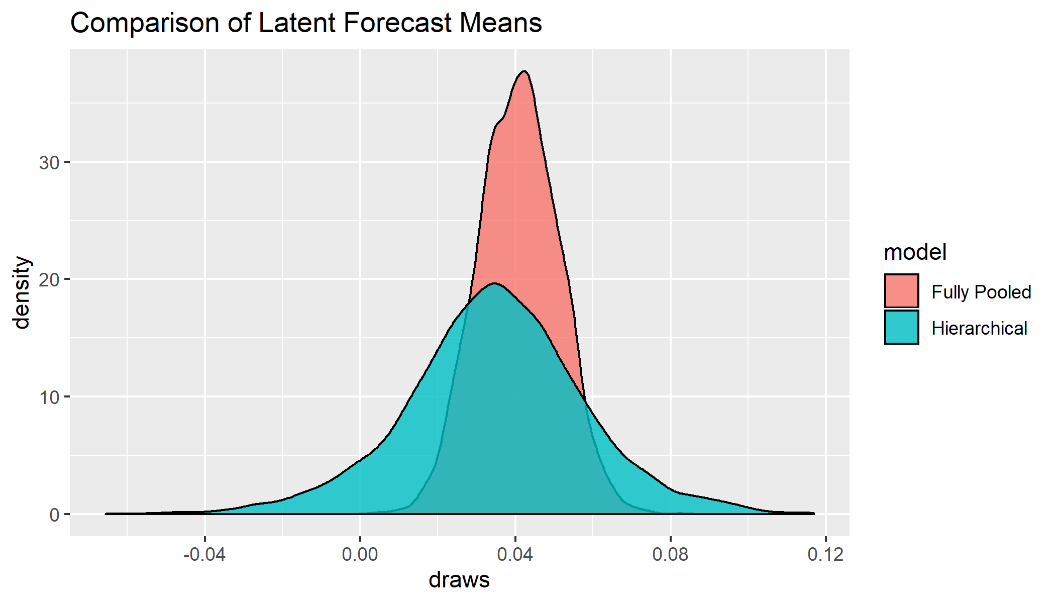
This is telling us that on average we should expect a log return of 0.036, corresponding to a 3.5% return, with a 95% posterior interval between -1.3% and 7.8%. This point prediction will be fairly close to a weighted average of the various analyst forecasts, but what is quite different is the level of uncertainty associated with the model.
If we ignored the two-level nature of the problem and just pooled together the observations toward the mean, we would firstly be ignoring that some analysts are more confident than others, and secondly that there is uncertainty associated with the underlying measurements.
We can compare exactly this with baggr’s baggr_compare method.
pooling_comparison <-
  baggr_compare(us_eq_forecasts,
              prior_hypermean = normal(0.08, 0.2),
              prior_hypersd = cauchy(0, 0.05),
              control = list(adapt_delta = 0.9),
              what = "pooling")
We can see even with the same priors, the full pooling model is both more bullish and more certain because it is ignoring the underlying uncertainty of the measurements!
Mean treatment effects:
           2.5%   mean  97.5%
none         NA     NA     NA
partial -0.0134 0.0347 0.0820
full     0.0213 0.0408 0.0608

SD for treatment effects:
          2.5%   mean  97.5%
none        NA     NA     NA
partial 0.0107 0.0452 0.0996
full    0.0000 0.0000 0.0000
The variance in forecasts for the fully pooled model only takes into account the heterogeneity of the measurements, not the certainty of the analysts. We can see the discrepancy by plotting posterior draws for $\tau$ from both models.
Obviously this is just aggregating means, but I believe a similar method could be use to aggregate full covariance matrices across different firms. It could also be useful for aggregating outputs of a mix of quantitative and qualitative models (or purely quantitative models that lack a track record).
This also assumes that we know essentially nothing about the relative quality of the analysts or the correlation of their forecasts. If analysts herd, as they seem to do, we likely also want to take into account the correlations of their forecasts in generating our posterior. We could even model expected variance as a forecasted random variable! But I’ll leave all that for a future post.